ML&DL Notes: Learning Theory

Let $\mathcal{X}$ is the input space, and $\mathcal{Y}$ is the output space. Labeled example: $(\mathrm{x}, y)\in\mathcal{X}\times\mathcal{Y}$ . Interpretation:

• $\mathrm{x}$ represents the description or measurements of an object;
• $y$ is the category to which that object belongs.

Loss

Assume there is a distribution $\mathcal{D}$ over space of labeled examples $\mathcal{X}\times\mathcal{Y}$.

• $\mathcal{D}$ is unknown, but it represents the population we care about;
• Correct labeling function: $f: \mathcal{X}\rightarrow\mathcal{Y}$ and that $Y=f(X)$;
• We define the Loss of the classifier $h$

$$L(h(X), f(X)) = L(h(X), Y)=\left\{ \begin{array}{lr} 1,& \mathtt{if}\ h(X)\neq Y\\ 0,& \mathtt{if}\ h(X) = Y \end{array} \qquad 0-1\ Loss \right.$$

True Risk

The true risk of a classifier $h$ is the probability that not predict correctly on $\mathcal{D}$

$$R_{\mathcal{D}}(h):= \mathbb{P}[h(X)\neq f(X)] = \mathbb{P}[h(X)\neq Y]$$

In other words, the true risk is the expected value of the loss

$$R_{\mathcal{D}}(h):=\mathbb{E}_{X\sim\mathcal{D}}\{L(h(X), Y)\}$$

Bayes Classifier To find $h:\mathcal{X}\rightarrow\mathcal{Y}$, we try to minimize the True Risk $\mathbb{P}[h(x)\neq y]$, such that $h(x)=\mathop{\arg\max}\limits_{y\in\mathcal{Y}}\ \mathbb{P}[Y=y|X=x]$ As we already know, this is Bayes Classifier.

Bayes Risk

Donate by $h^*$ the Bayes classifier

• For the Bayes Risk $R_{\mathcal{D}}(h^*)$ it holds $R_{\mathcal{D}}(h^*)\leq R_{\mathcal{D}}(h)$ for any $\mathcal{H}$ and $h\in\mathcal{H}$, where $\mathcal{H}$ refer to the set of all possible classifiers.
• You cannot improve over the Bayes Risk.

Batch Learning

We do not know $f$ and we need to estimate $h$ from the data

• Learner’s input: Training data $S = \{(x_1, y_1)\dots(x_m, y_m)\}\in (\mathcal{X}\times\mathcal{Y})^m$
• Learner’s output: A prediction rule $h:\mathcal{X}\rightarrow\mathcal{Y}$ The goal of learner is that h shoud be correct on future examples.

IID condition

Key assumption: an i.i.d.(identically and independently distribution) sample from $\mathcal{D}$. This assumption is the connection between what we've seen in the past and what we expect to see in the future.

Empirical Risk

Calculate Empirical Risk by benchmarking the prediction against ground truth:

$$R_S(h) = \frac{1}{m}\sum^m_{i=1}\mathbb{I}[h(x_i)\neq y_i]$$

where $\mathbb{I}$ is the indicator function means the Loss function here is 0-1 Loss.

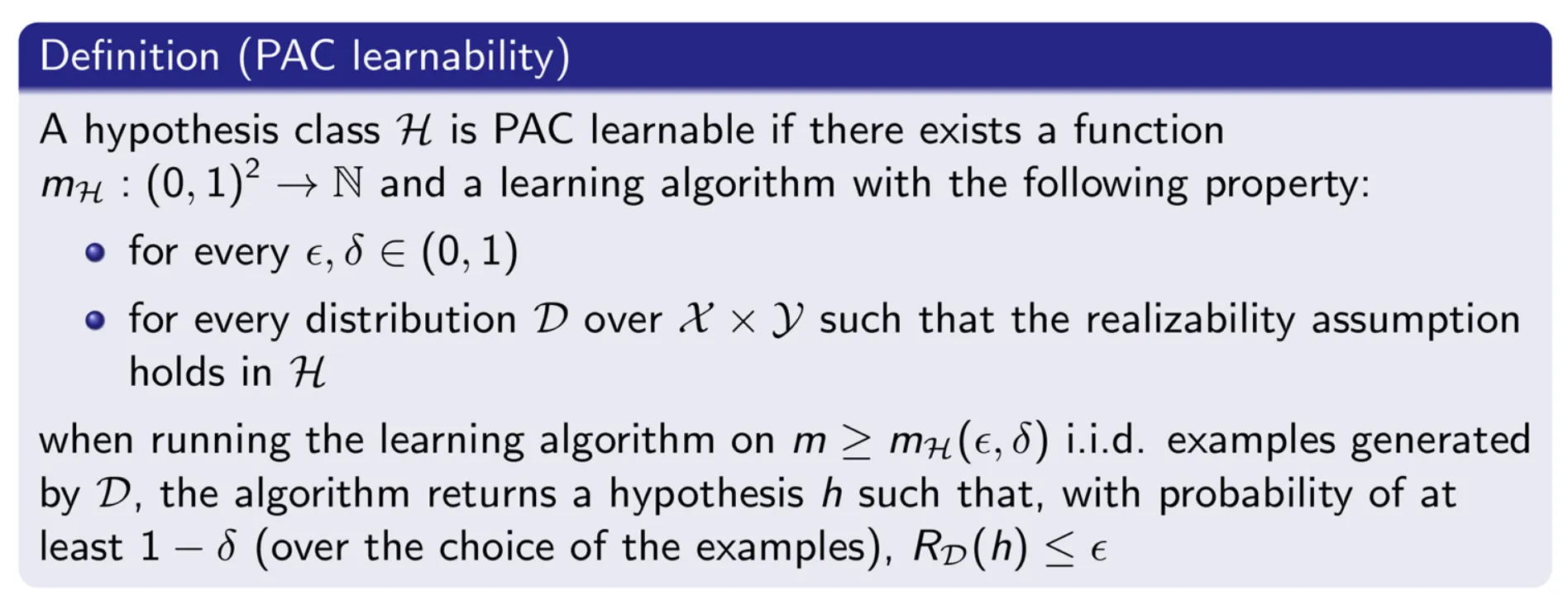
Probably Approximately Correct (PAC) Learning

Can Only Be Probably Correct

Claim: Even when $R_{\mathcal{D}}(h^*)=0$, we can’t hope to find $h$ s.t. $R_{\mathcal{D}}(h)=0$. Relaxation: $R_{\mathcal{D}}(h)\leq \epsilon$, where $\epsilon$ is user-specified

Can Only Be Approximately Correct

Claim: No algorithm can guarantee $R_{\mathcal{D}}\leq \epsilon$ for sure. Relaxation: Allow the alg. to fail with probability $\delta$, where $\delta\in(0,1)$ is user-specified.

1. The learner doesn’t know $\mathcal{D}$ and Bayes predictor $h^*$.
2. The learner specifies the accuracy parameter $\epsilon$ and confidence parameter $\delta$.
3. The number of examples can depend on the value of $\epsilon$ and $\delta$, which we call it $m(\epsilon, \delta$); but not depend on distribution $\mathcal{D}$ or Bayes function.
4. Learner should output a hypothesis $h$ s.t. $\mathbb{P}[R_{\mathcal{D}}\leq\epsilon]\geq1-\delta$.

That is PAC Learning.

Realizability Assumption

Assume that, for a given class $\mathcal{H}$ of functions $f:\mathcal{X}\rightarrow\mathcal{Y}$, there exists $h^*\in\mathcal{H}$ such that $R_{\mathcal{D}}(h^*)=0$, which implies that $h^*$ is the Bayes classifier.

$m_{\mathcal{H}}$ is called the sample complexity of learning $\mathcal{H}$.

PAC Learnability 的核心思想是：如果一个假设类是 PAC Learnable，意味着我们可以通过有限数量的样本来学到一个接近最优的假设，并保证其泛化误差可控。

With more constraints, 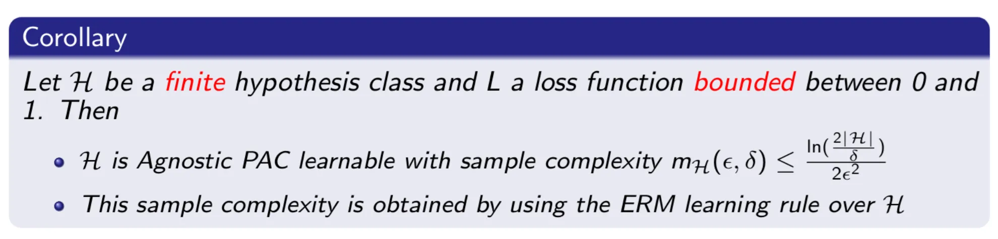for example, the “0-1 Loss” is okay for that, but square Loss isn’t because it not bounded.

Shattering & VC-dimension

Which are the important concepts to measure complexity of hypothesis space. 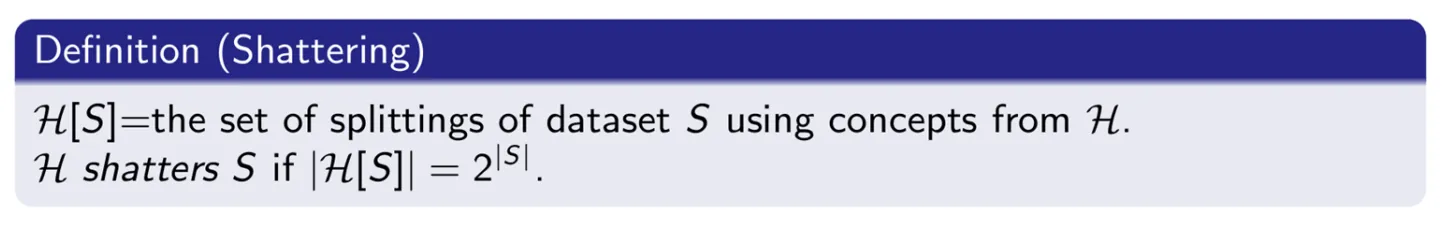对于一个假设集合（Hypothesis Class）$\mathcal{H}$，如果它能够在一个大小为 $m$ 的数据集上实现所有可能的二分类标记方式，那么我们说 $\mathcal{H}$ shatter[v.粉碎] 了该数据集。i.e. 假设有一个二分类模型（例如直线分类器）和一个数据集，如果能找到某种参数设定，使得该模型能够对数据点的所有可能标签分配方式都正确分类，则称该模型 shatter 了这个数据集。

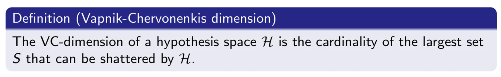假设空间 $\mathcal{H}$ 的 VC 维度（ VC($\mathcal{H}$) ）是 $\mathcal{H}$ 可以粉碎的最大数据点数。

In order to prove that $VC(\mathcal{H})$ is at least $d$, we need to show only that there’s at least one set of size $d$ that can be shattered by $\mathcal{H}$.

Linear Classifier

Consider $\mathcal{H}$ as the set of linear classifiers in $d$ dimensions, then $VC(\mathcal{H}) = d+1$.

Not PAC Learnable

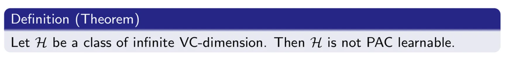
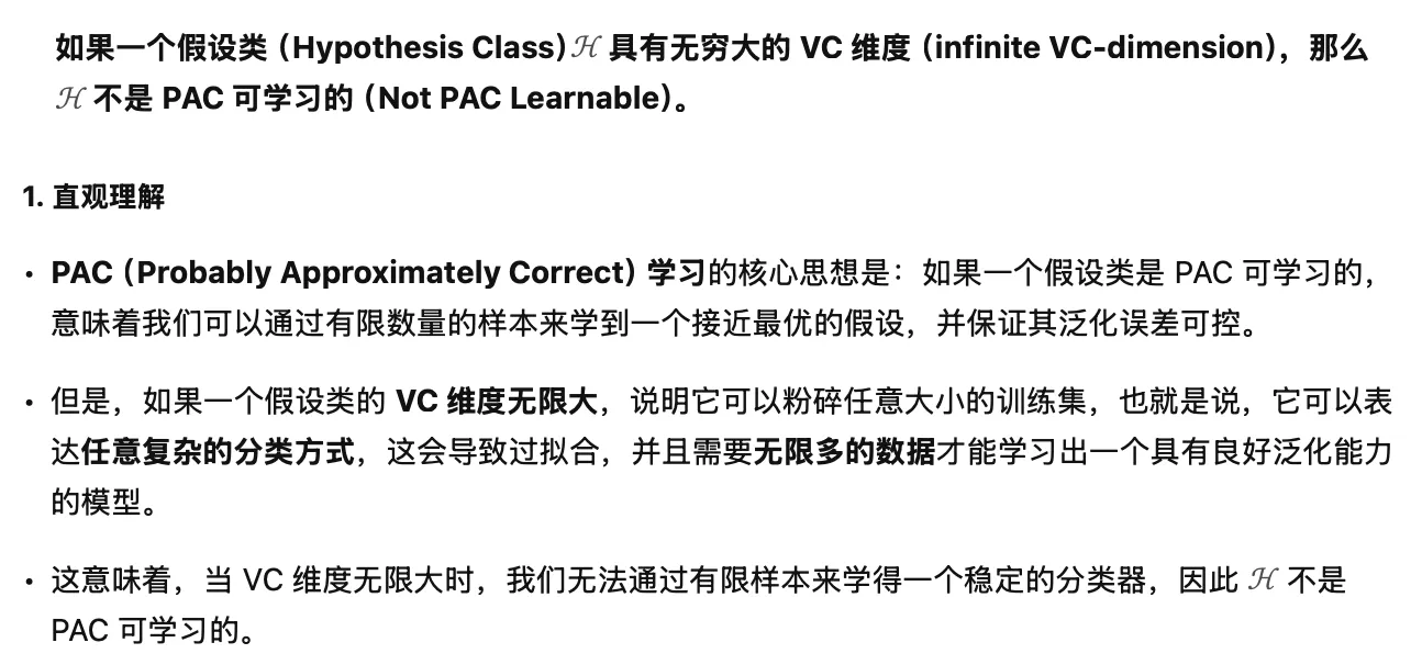
Infinite Hypothesis Classes

• 理论上，假设类可以是无限的，但计算机实现时会受限于离散化存储，任何模型参数都是以浮点数存储的，对于$32\ \mathrm{bits}$ 的浮点数就只有 $2^{32}$ 种可能的取值，因此假设类在计算上是有限的。
• 对于具有 $d$ 个参数的模型，假设类的大小可以估计为 $2^{32d}$，并且经验法则告诉我们，至少需要 $10d$ 个样本来有效训练模型。

Overfitting

The model has pretty excellent performance on the training set, but poor performance on the test data or the real world.

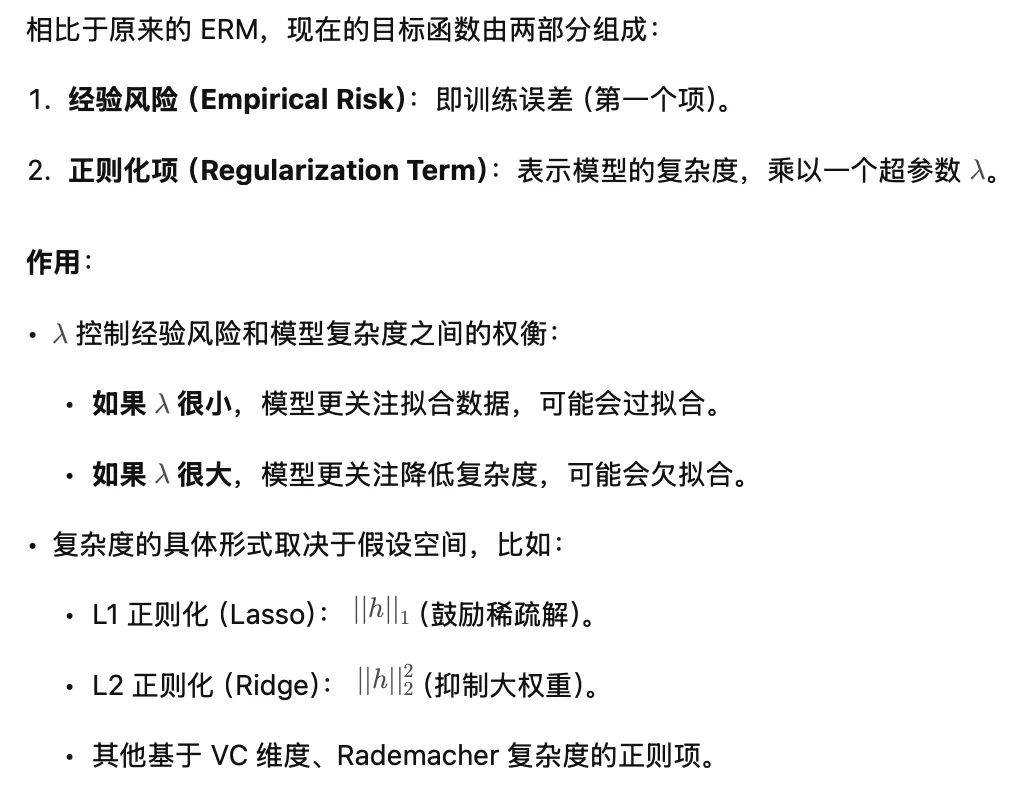
Regularization ERM (Empirical Risk Minimization)

$$h_S = \mathop{\arg\min}\limits_{h\in\mathcal{H}}\left(\frac{1}{m}\sum_{i=1}^m\mathbb{I}[h(x_i)\neq y_i]+\lambda\ \mathrm{Complexity}(h) \right)$$